Understanding the Timestamp

This is an explanation of how the timestamp work in data collected on a PC via the Bitbrain Data Viewer.  This data could come from the Versatile Bio, and any of the Minimal or Versatile EEG systems. 

This is not relevant for data exported by SennsLab (where a script automates this process), or saved to the SD card directly (where there is no PC-based timestamp).

Data Transmission Method

The amplifier is connected to the PC via Bluetooth.  This has the advantage of allowing the participant freedom of untethered movement.  However, there are some limitations due to bandwidth and accuracy that have to be accounted for when analyzing data. 

The amplifier collects data at 256 samples per second.  Rather than transmit this in full, which would potentially exceed BT bandwidth, the amplifier transmits these samples in packets, or blocks, of 8 samples each, 32 times per second. 

Timestamp and Sequence

When the PC receives this block of 8 samples, the block itself is stamped according to the CPU clock time, and then numbered consecutively.  When viewing the data, it looks like this:

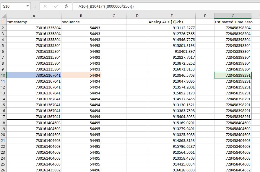
This is an example data file from the Versatile Bio, showing the Aux input channel (in this case attached to a GSR sensor). 

Each line is a sample is recorded at 256 Hz, but organized into blocks of 8 samples that are each timestamped and numbered consecutively by the PC when received.  In the data file:

• Timestamp = the time assigned to the block of data by the CPU, in microseconds.  In this case, the 8 samples in block 1 have a timestamp of 730161335804 microseconds.
• Sequence = a consecutive number for each block of data.  Block 1 is numbered 54493
• Analog AUX [1]-ch1 = This is data from the specific input on the amplifier (the name will change depending on the system and channel viewed). 

Delays and Missing Samples

There are three conditions that can effect the accuracy of the recorded timestamp and the transmission of data:

1. There is a time of flight delay corresponding to the transmission time of the Bluetooth signal, which is basically consistent and estimated to be 40 ms.  
   
2. There is a variable delay called jitter which is basically a randomized inaccuracy in the receiving time caused by a number of factors, typically in a range of +/- 10 ms
3. There is the potential for missing samples, usually caused by the participant temporarily leaving the Bluetooth range, or possibly caused by interference in BT frequencies. 

These limitations have to be accounted for when calculating a corrected timestamp.  This corrected time stamp then has to be applied to all blocks in the data file (32 per second) and then extrapolated to each sample in the block (256 per second).  After this, we'll have a data file with a proper timestamp that is corrected for all 3 issues above.

Step 1:  Remove jitter from start time value

Because jitter is a randomized source of error, it can be accommodated by using multiple block timestamps to calculate what the start time of the data file is predicted to be based on the block sequence, and then finding the median value to predict the correct starting timestamp for block 1.  

For example, in the first block of our data, the timestamp  is listed as 730161335804 microseconds, block number 54493.

For the second block in our data, the time stamp is listed as 730161367041 microseconds and this is block number 54494.  This block should be time stamped exactly 1/32 seconds (31.25 ms) after the first, since the blocks are sequential and transmitted 32 times per second.  But because of the random jitter introduced by the Bluetooth transmission, it isn't.  If we subtract the timestamp of block 54493 from 54494 we get a difference of 31.237 ms.  (This is not a huge error but jitter is random and can be much higher on other samples in the data file).

Using a simple formula, we can use the any block to predict what the correct start time was for the data file.  The formula looks like this:

Jitter_corrected_start_time= block_time_stamp - [(block_number + 1) * (31250)]

We will apply this formula to the second block of data, shown here (outlined in black):

In excel, this formula is:

=A10-((B10+1)*((31250)))

The block_time_stamp is the uncorrected timestamp applied to the block in question, in this case 730161367041 microseconds, marked blue in the picture.   

The block_number is the sequence number corresponding to the ordered number for this block, in this case 54494, marked red. 

The value 31250 corresponds to the sample period of the amplifier transmission in microseconds (1/32 seconds).  The actual sample rate is 8 times higher, but the amplifier sends 8 samples per packet. 

Applying this formula for the second block of data calculates a predicted start time of 728458398291 microseconds - as predicted by this block of data, marked green. 

Applying the formula to the third block of data calculates a predicted start time of 728458404603. 

By applying this formula to a significant number of blocks of data, we can calculate a median value for start time that will eliminate the jitter from the start time calculation.  Since this error is random, we can assume it averages out to zero over time. 

In our case, we've applied this formula for each sample, then calculated the median of these values.  The formula to do this in excel is simply:

=MEDIAN(G:G)

This comes out to a jitter-corrected start time of 728458405035 microseconds, as estimated from all of our data samples.

Step 2:  Correct for time of flight

The jitter-corrected start time does not include the time of flight for Bluetooth transmission.  This is a fixed value which we estimate at 40 ms, or 40,000 microseconds.  This will have to be subtracted from the timestamp in order to determine the actual time of the event recorded by the amplifier. 

Simply subtract that number from the corrected start time.  We now have a value of 728458365035 for the corrected_start_time of the recording.

Step 3:  Calculate corrected timestamp for all blocks

Now that we have a corrected value for the start of the recording, we can calculate the corrected time stamp for each 8-sample block.  To do this we apply the following formula:

Corrected_block_timestamp = corrected_start_time + (sequence * 31250)

Where sequence is the incremental number of the block, corrected_start_time is the final value from step 2, and 31250 is the 32 Hz sample period (time between blocks) in microseconds. 

Applying this to our data, looks like this:

In excel, the formula for the highlighted cell looks like this:

=728458365035+(B10*31250)

Where 728458365035 is the corrected start time calculated in step 2.

This formula calculates the corrected timestamp of each block of data by using the corrected start time and adding a time interval based on the number of samples that have happened since the start of recording.  Additionally this will accommodate missing blocks of data since the corrected timestamp is calculated based on the sequence value of blocks.  If any are missing, they will be skipped in the sequence and not considered when calculating the timestamp.  There will be a gap of time with no data in this scenario. 

Step 4:  Calculate the timestamp for each sample

Now we have a corrected timestamp for each block of data, which is correct for the first of the 8 samples in the data block.  We simply need to extrapolate this through the other 7 samples by the true sample rate of 256 Hz.  Add 1000000/256 or 3906.25 microseconds to each consecutive sample in the block after the first one (but only calculated for that block). 

On our data:

The first cell in the block is correct and set to the adjusted block time.  In excel for block K10 this looks like:

=I10

For K11, the second sample of the block, the formula is:

=K10+3906.25

And so on, until all 7 additional samples have an assigned timestamp.  Then repeat these 8 formulas for each cell in all subsequent blocks. 

You now have a timestamp that is corrected for jitter and time of flight, and extrapolated to all samples in the 256 Hz data file. 

This process is the same for all data files recorded by the Versatile Bio, Minimal EEG or Versatile EEG systems.  This routine can be created as a script in Matlab or Python, or as a worksheet in in Excel and applied to all data files.  Some examples of this are available, contact Bitbrain support for more information.